Image Recognition with Neural Networks: A Beginner’s Guide
Jul 19th, 2024 | 16 min read
Table Of Contents
- Building Blocks of Images: Pixels and Patterns
- What’s a Neural Network?
- Pattern Recognition through a Neural Network
- Running the Detection Algorithm
- The Secret Sauce: Weights and Biases
- Learning from Mistakes: Gradient Descent
- Beyond Simple Patterns: Scaling up
- Neural Networks: Features and Challenges
- Types of Neural Networks
- The Future of Image Recognition
- Questions and Answers
If you’re anything like me, you must be anxious to understand how computers can recognize image. Certainly, it can’t be magic—we know that for a fact—but how does it work?
As a disclaimer, I’m not a neural network expert. I love to learn and share my knowledge and experience. Hence, the following example is more like a “hello world” of image recognition. I’m also not a math genius, which means that if I can understand how math works, everyone can!
That said, don’t worry if you’re new to image recognition based on neural networks. We’ll start with the very basics and work our way up. By the end of this blog post, you will understand how computers recognize the simplest patterns.
Building Blocks of Images: Pixels and Patterns
Starting at the very beginning, let’s talk about images and how computers look at them. I guess most people will know about pixels. Pixels are a single point in an image, defined by a color and its position.
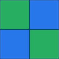
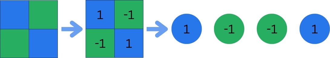
If we look at the example to the left, we can see a very simple image made up of (ignore the zooming) four pixels: two blue and two green, each color spread diagonally.
If we want to describe these pixels in a slightly more technical fashion, we could assign a number to the different colors. Let’s say blue=1 and green=-1.
That way, we can write this image as a sequence of four numbers, going left to right and top to bottom. 1, -1, -1, 1
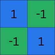
If you find it hard to grasp, no worries. Bringing it back to our pixel image, we can place the numbers right on the different pixels to make it more clear. I hope it makes more sense now.
The idea here is simple: we want to mathematically describe what we see. In reality, the numbers would either represent the actual color (HDR has more than one billion colors) or a range of colors represented using a single number (like when we grayscale images).
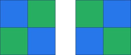
Since we have defined the basics of the math of our pattern recognition, what are the patterns we could recognize? Well, we only have four pixels and two colors, but we want to keep it simple, don’t we?
Anyhow, our options are the following two patterns. One starts with green in the top-left corner, and the other one starts with blue respectively.
What’s a Neural Network?
Before we start implementing our own neural network, we should clarify what a neural network actually is. At its core, a neural network is a series of chain mathematical operations. Neural networks are directly inspired by how our brain works, hence the name.
Anyhow, a neural network is a web of interconnected “neurons” (just like our brain) that interact, process, and pass along information between each other.
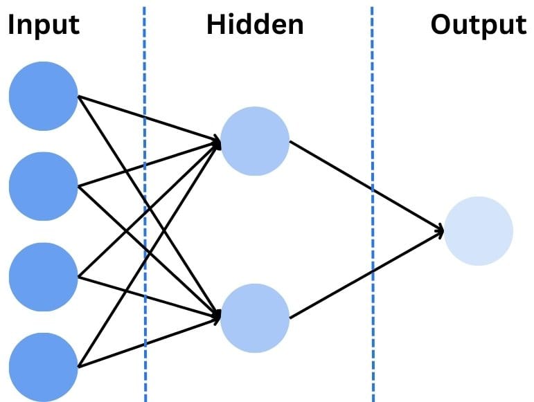
Those neurons are separated into a set of layers. Normally, experts speak of three layers:
- Input Layer: the input data (four pixels)
- Hidden Layer: the mathematical magic
- Output Layer: the result of the network
In our example, the number of input elements is finite. That means that the hidden layer, the actual magic, can be simple and easy to understand. The output layer would be the recognized image if it was able to recognize it.
For simplicity, we only want to teach it to recognize if there is a diagonal color shift between green and blue. Meaning, that anything other than the two above examples would fail to be recognized.
Pattern Recognition through a Neural Network
When building a neural network, we have to start with some kind of input. In our case, we have a set of eight images, each four pixels with a combination of our two colors
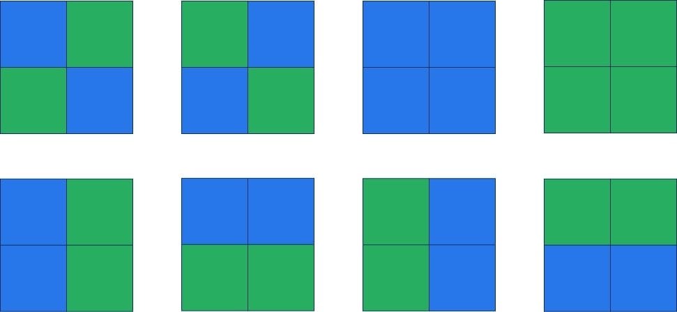
Whatever we build, it should only recognize the first two images. Images the first two images to build pictures of cats, whereas the remaining ones are boring snails (not judging anyone who loves snails, just saying!).
The Input Layer
Our first step is to build out the input layer. To represent our image, we need four neurons as input. You can think of those neurons as properties of any kind.
Imagine you want to figure out if a room needs cleaning. In this case, we wouldn’t have four pixels but many 4 properties related to room cleaning, such as Is the room already clean? Is it a storage room? (Storage rooms are never cleaned; ask your attic!) Do I actually own a hoover? Finally, is there a power outage ongoing that would keep me from hoovering?
Anyway, coming back to our four pixels, we would represent them as a set of four input neurons.
The Hidden Layer(s)
The hidden layer receives input from the input layer. The hidden layer in itself can contain many steps. Actually, it is not uncommon to have many steps in the hidden layer. How many depends on how many parameters we want to analyze. In our case, we want to know exactly one property of the image. Is there a diagonal color shift or not?
That means, for this very simple example, our hidden layer will be a single mathematical function and results as the immediate result of our recognition function. But what mathematical magic should we use here?
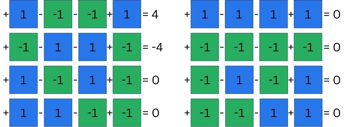
Actual neural networks may have more complex algorithms, but we want to stick to the very foundation of our mathematics, addition and subtraction.
Applying either of those two operations on each of the four input neurons, we have a potential of 16 combinations.
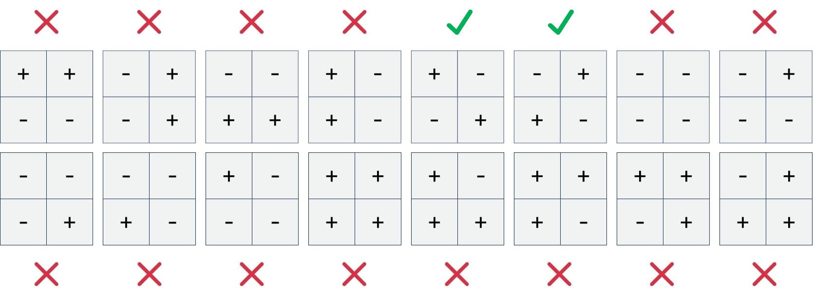
As you can see, the potential candidates are also marked as working or not. Working, in this case, means that the calculation would yield distinguishable results for our set of eight input images.
The two candidates we could use look weirdly familiar, just using symbols instead of our numbers. This isn’t always the case, but for this very simple example, with only one parameter, it makes sense. The pattern we want to recognize is the pattern that can be used to recognize it.
In reality, computers would be used to find the “best” combination of the candidates. Due to the exponential growth of the number of combinations, best is meant as a heuristic approach. Engineers would start from one combination and, in many iterations, adjust it ever so slightly, using one of the better results for the next iteration. At some point, they may stop and assume to be close enough to the “best” solution.
To show the exponential growth, here is a table of growth of either the number of pixels we want to recognize in a single run or the number of potential mathematical operations. The combinations run wild quickly.
| Available operations | Number of pixels | Possible combinations |
|---|---|---|
| 2 | 4 | 16 |
| 2 | 8 | 256 |
| 4 | 4 | 256 |
| 4 | 8 | 65536 |
| 8 | 8 | 16777216 |
| 8 | 16 | 281474976710656 |
Finally, each neuron passes is result to an “activation function”. The activation function is used to determine the output of the neuron. It receives the calculation result and applies some type of decision functionality. A little bit simplified, it decides whether the neuron is “activated” or not.
The Output Layer
The output layer combines the outputs from the hidden layer and calculates the final prediction. While the hidden layer may have many steps of calculations, the output layer is a single step.
In that set, the output layer has two primary uses:
- Final Decision Point: The output layer is where the network’s final decision is made. After the data passes through the hidden layers (and the input layer, for that matter), the output layer processes this information to generate the final output.
- Result Interpretation: The output layer translates the network’s internal representation into a format to be understood by humans. This can be a simple output like 0 or 1, true or false, but also more complex outputs such as probabilities, classification, regression results, or similar.
In our simple example, the output will be classified by a simple comparison if the final output is equal to zero (unrecognized), below zero (top-left, bottom-right), and above zero (top-right, bottom-left). Not the most amazing of all classifications, but it is what we set out to achieve 🤷♂️.
Running the Detection Algorithm
Now that we know the basic concepts, it’s time to try and run the first iteration of our neural network and see how it would process our 4-pixel images.
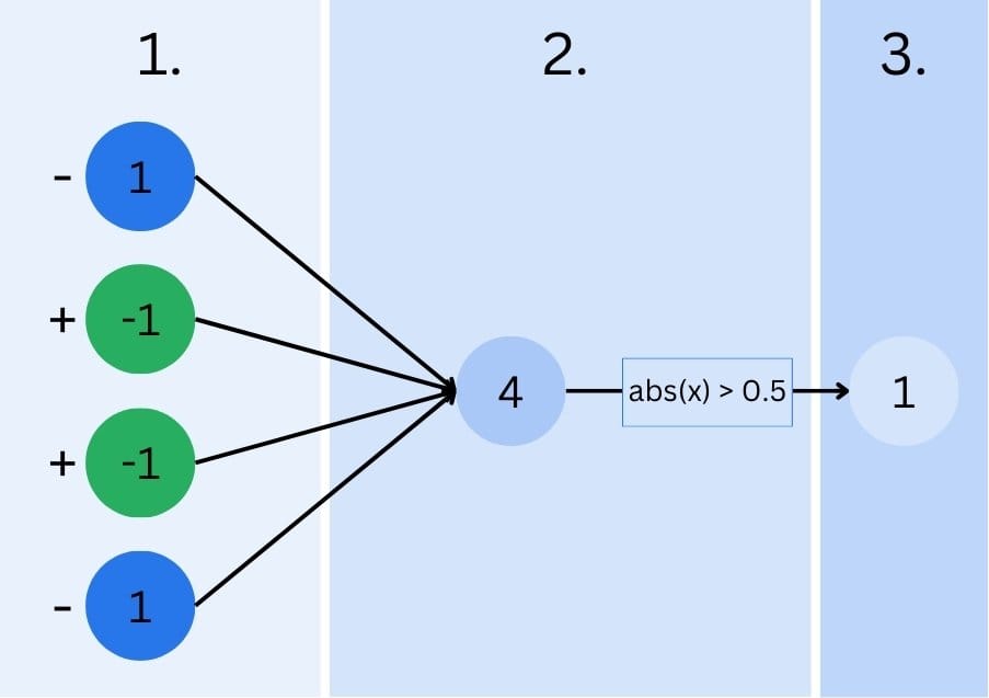
- Input Layer: Each pixel’s value ( -1 for green, 1 for blue) is fed into the network.
- Hidden Layer: Each neuron in this layer receives inputs from all four pixels, does some additional magic (we’ll talk about it in a second and ignore it for now), and then applies an activation function to determine its output. In our simple case, the activation function tests the neuron’s output to unequal zero. Zero means that no diagonal color switch is detected, one means our neural network found one.
- Output Layer: This layer combines the outputs from the hidden layer to make a final prediction. In our case, it might output a value close to 1 for a top-left to bottom-right diagonal and close to 0 for the other diagonal.
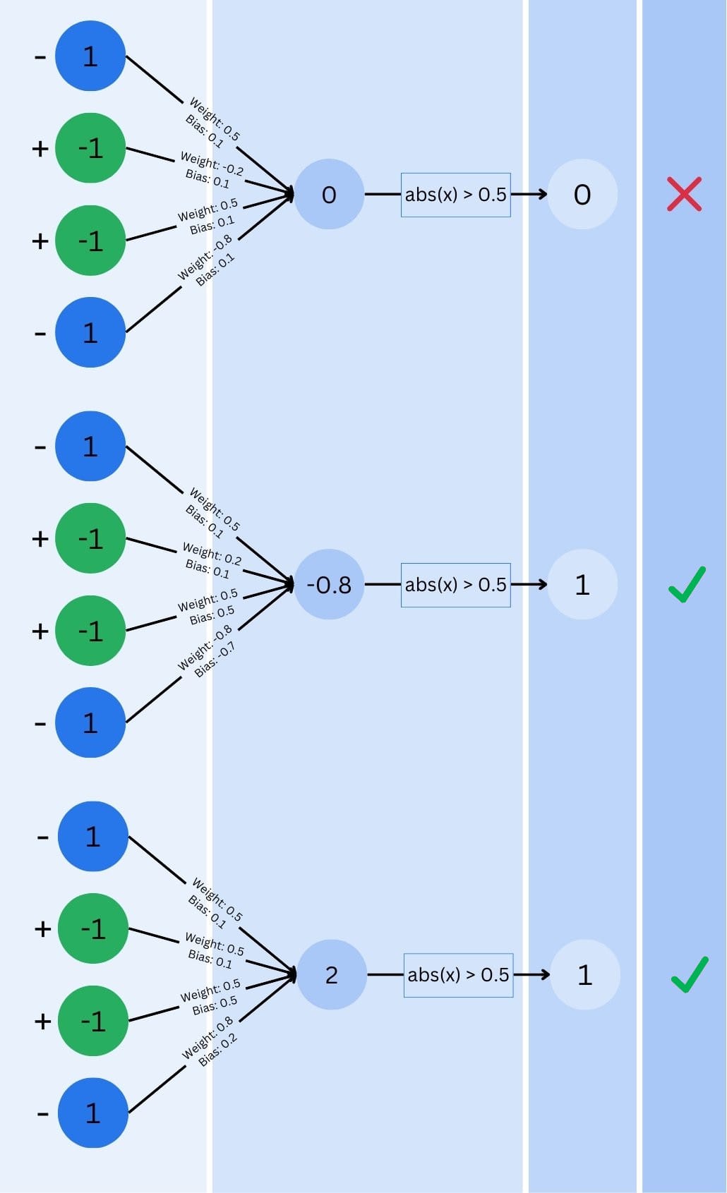
The Secret Sauce: Weights and Biases
Now, so far, I kept one important piece of information away from you. Each connection between neurons has a “weight” associated with it. These weights determine how important each piece of information is. Additionally, each neuron has a “bias” – think of it as the neuron’s tendency to fire regardless of its inputs.
The network starts with random weights and biases. When training the neural network, you push many different test inputs through the neurons and compare the result to a predefined one. According to the result (whether the dog was recognized or not), the neural network will adjust its weights and biases, optimizing itself for better-recognizing patterns. But how does the network training know how to adjust them? That’s where our next concept comes in.
Learning from Mistakes: Gradient Descent
Imagine you’re blindfolded and trying to find the lowest point in a hilly area. You’d probably take small steps, feeling the ground beneath your feet to determine if you’re going downhill or uphill. This is essentially what gradient descent does for our neural network. At least, this is how Andrew Ng explains it in this Coursera session on Machine Learning.
The network makes a prediction, compares it to the correct answer, and then adjusts its weights and biases to reduce the error. It does this over and over, gradually improving its accuracy. This is the process called “training”.
The more images we pass during the training phase, the better the model tends to be. After the training, the model configuration is exported and can be loaded into other devices (such as mobile phones). Training the model typically requires quite massive storage systems and compute resources, running millions and billions of training images. Remember, we’re just using one parameter here, actual neural networks have tens of thousands to hundreds of thousands, and sometimes even millions of them.
Beyond Simple Patterns: Scaling up
Now, that was cool. Tap yourself on your shoulder. You’ve built your first neural network. Celebrate it. Put Artificial Intelligence as a skill to LinkedIn 🤣
How can we add additional features and keep growing this network? What about a network that could differentiate between the blue diagonal line starting at the top or the bottom left? It’d be easy to do. We now know that there are weights, so we may be able to utilize them.
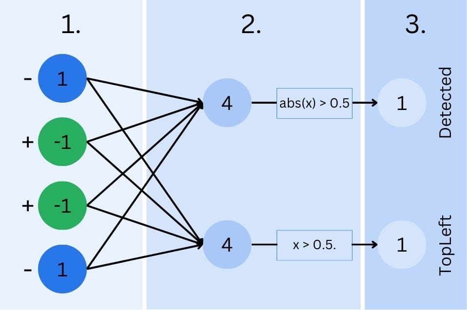
To achieve this, we add a second output. The first one will still fire every time an image is recognized, while the second output will only fire if the first pixel is blue. Using those two outputs, we can conclude if we detected a diagonal line and if we have a green or blue diagonal line starting top-left (binary choice).
Anyhow, while our basic, 4-pixel example is a great starting point, real-world image recognition is much more complex. Modern neural networks used for tasks like facial recognition or object detection in photographs use millions of parameters and are trained on massive datasets. In fact, modern neural networks don’t just recognize images-they can even unpixelate image by predicting and reconstructing details that are not visible in the original, low-resolution version. However, the fundamental principles remain the same.
Neural Networks: Features and Challenges
One of the most powerful aspects of neural networks is their ability to learn features automatically. In our simple example, the network might learn to pay attention to specific pixel combinations that indicate a diagonal line.
In more complex networks, early layers might learn to detect edges or simple shapes, while deeper layers combine these to recognize more complex patterns like faces or objects. Experimenting with AI-generated visuals can also support training models to identify a broader range of object variations and patterns. This hierarchical learning is what makes neural networks so effective for image recognition tasks.
However, while neural networks are powerful, they’re not without challenges:
- Overfitting: Sometimes, a network becomes too specialized in its training data and performs poorly on new, unseen examples.
- Computational Resources: Training complex networks requires significant computing power and time.
- Storage Resources: Training data sets require vast amounts of high-throughput storage to keep up with current and next-gen GPU-based training setups.
- Data Quality and Quantity: The old saying “garbage in, garbage out” applies here. Networks need large amounts of high-quality, diverse data to learn effectively.
- Interpretability: Unlike simpler algorithms, it can be difficult to understand exactly why a neural network made a particular decision.

Types of Neural Networks
While we talked about neural networks as if there is only one type, this isn’t actually true though. There are many different approaches to neural network-based deep learning. However, three specific types are most prominent, with many modern applications using hybrid approaches, combining different types of neural networks to leverage their respective strengths.
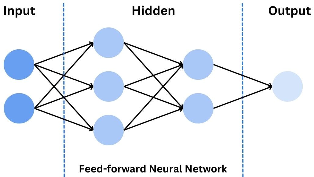
Feed-forward Neural Networks (FNN or FFNN)
The simplest type of neural network, and the one we’ve been using in our 4-pixel example, is the feed-forward neural network, abbreviated as FNN. In a feed-forward neural network, information flows in only one direction: from the input layer, through the hidden layer(s), to the output layer. There are no loops or cycles in the network.
FNNs are great for simple classification tasks. They are also a great way to serve as the foundation for understanding more complex networks.
They have, however, limitations when it comes to processing sequential data or capturing spatial relationships in images. That said, while they can be used for image recognition (as we did above), the use cases are normally limited to very simple images.
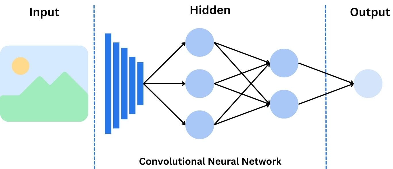
Convolutional Neural Networks (CNN)
When it comes to image recognition, convolutional neural networks are the stars of the show. Convolutional neural networks (commonly abbreviated as CNNs) are specifically designed to process grid-like data, such as images (pixel grids).
The key feature of CNNs is the convolutional layer, which applies filters (or kernels) to detect features like edges, textures, and shapes. As the network deepens, it can recognize more complex patterns, making CNNs exceptionally good at tasks like object detection and facial recognition.
Convolutional neural networks are the workhorses of image recognition. They have an amazing ability to encode complex spatial patterns into hierarchical feature representations.
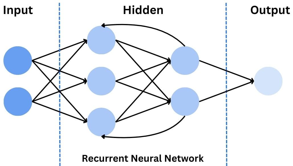
Recurrent Neural Networks (RNN)
The last large approach is the recurrent neural network or RNN.
While not typically used for static image recognition, RNNs are worth mentioning due to their importance in processing sequential data. RNNs have loops that allow information to persist, making them ideal for tasks involving time series or sequence prediction.
In the context of computer vision, RNNs can be useful for video analysis, where the temporal relationship between frames is important. They can also be combined with CNNs to create powerful models for tasks like image captioning or video classification.
The Future of Image Recognition
In this blog post, we covered a lot of groundwork, from the basics of how neural networks process information to gradient descent as the most common approach to training a neural network.
While our initial example was simplistic, it illustrates the fundamental concepts that underpin even the most advanced image recognition systems. Whether you’re dealing with four pixels or four million, the core ideas of weights, biases, and learning through error correction remain the same.
As the world continues to refine neural network architectures and training techniques, the capabilities of image recognition systems are expanding rapidly. From mobile phone apps, over medical diagnosis to autonomous vehicles, the applications are vast and growing.
That said, image recognition will increase in importance because “if we want machines to (be able to) think, we need to teach them to see,” as says Fei-Fei Li. I really recommend watching her TED talk. Towards the end, she explains, “It has been a long journey. To get from age zero to three was hard, but the real challenge is to go from age three to 13 and far beyond.” And who would know if not her?
So the next time you unlock your phone with facial recognition or see a self-driving car navigate traffic, you’ll have a better appreciation for the neural networks working behind the scenes. And if you build your own neural network and require a storage solution for your training data set, simplyblock is here to help.
Questions and Answers
Image recognition with neural networks refers to using deep learning models, especially convolutional neural networks (CNNs), to identify objects, patterns, or features in images. These models learn from large datasets and are widely used in facial recognition, medical imaging, and autonomous vehicles
Neural networks process images through multiple layers that detect features like edges, shapes, and textures. Over time, the model learns to recognize complex objects by training on labeled image datasets. This makes them highly accurate for both classification and object detection tasks.
Training neural networks on large image datasets requires high IOPS and low latency to avoid bottlenecks. Using fast block storage like NVMe over TCP ensures that GPUs and CPUs stay fully utilized during training, leading to faster model convergence.
Yes, simplyblock supports Kubernetes-native storage optimized for AI/ML workloads. It offers high-performance volumes, dynamic provisioning, and encryption, making it ideal for teams running distributed training or inference jobs on Kubernetes clusters.
For ML pipelines, low-latency and high-throughput storage is essential. Solutions like software-defined storage with NVMe support are ideal for model training, dataset preprocessing, and fast checkpointing during experimentation.